Bootstrapping
How to use your data to get out of a tight spot
Peter Humburg
21 October 2021
The Problem

Bootstrapping

Working with what we’ve got
- Idea: We have sample from the population we want to study, can we just create more samples from that?
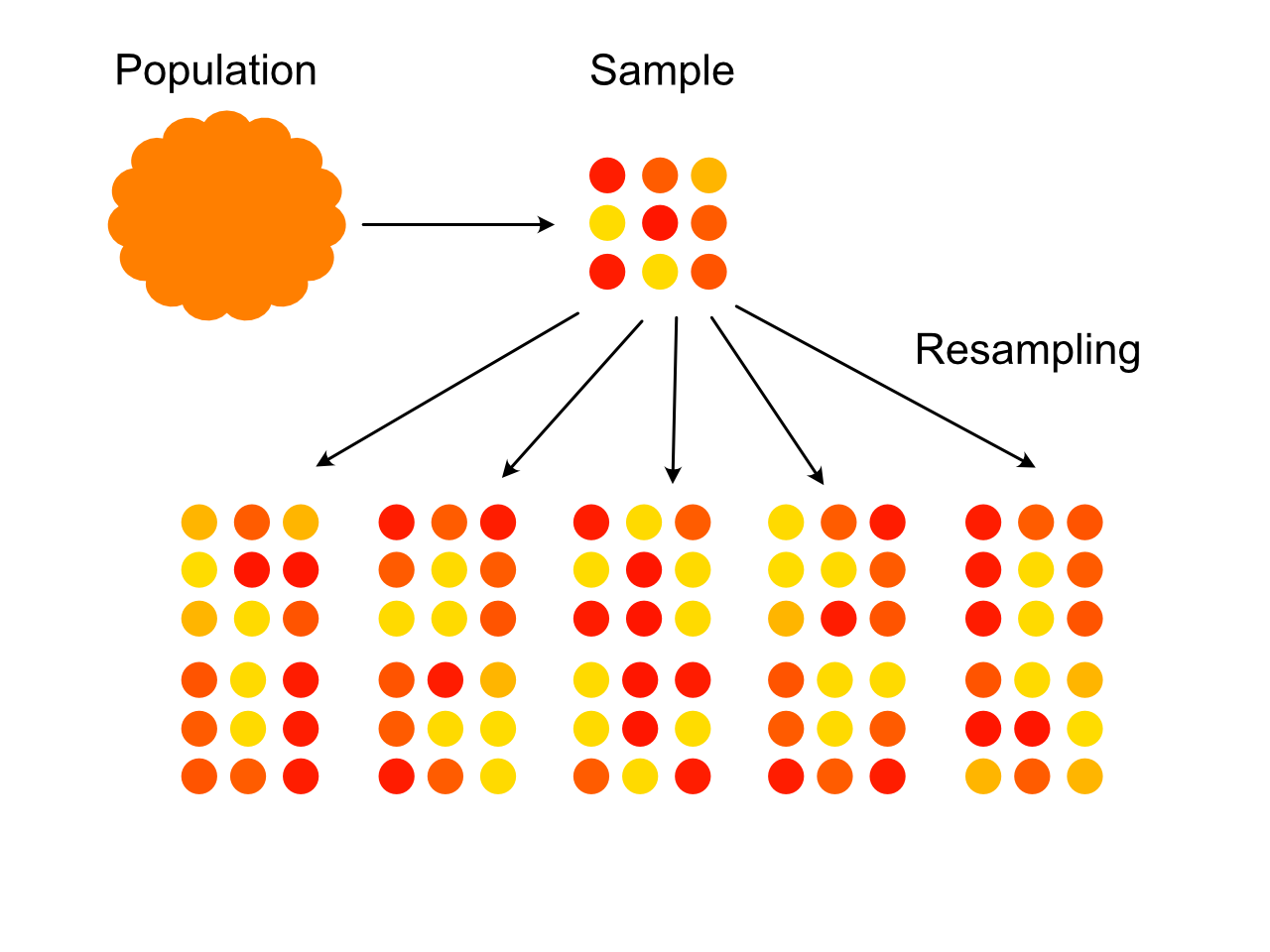
The Bootstrap
- Take a sample of size \(N\) from the population
- Compute sample statistic of interest \(S\)
- Randomly draw \(N\) observations with replacement from the original sample.
- Compute sample statistic \(S^*\) for this new sample.
- Repeat 2 - 4 many times.
Example: The speed of light
In 1882 Michelson and Morley measured the speed of light by timing a flash of light travelling between mirrors.
(reported here in km/s - 299,000)
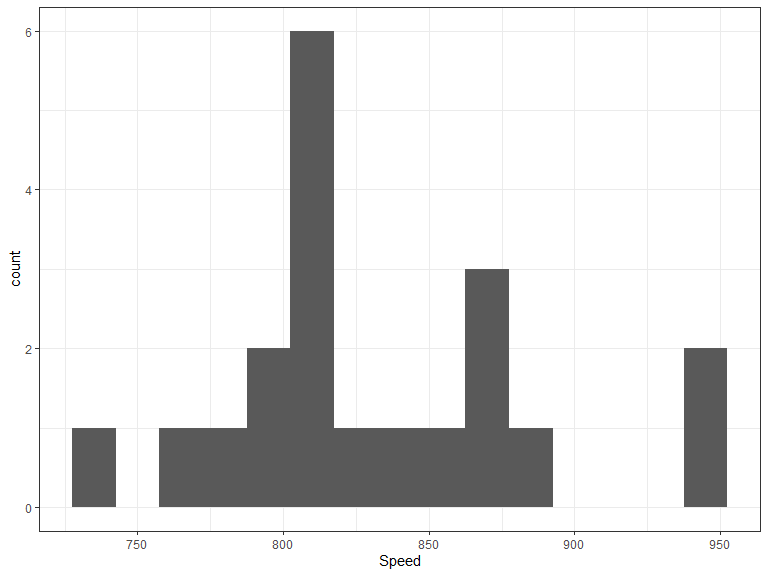
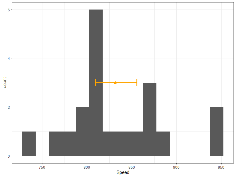
Estimating the speed of light
- 20 measurements taken
- Average observed speed of light is 831.5
- What would a 95% confidence interval look like?
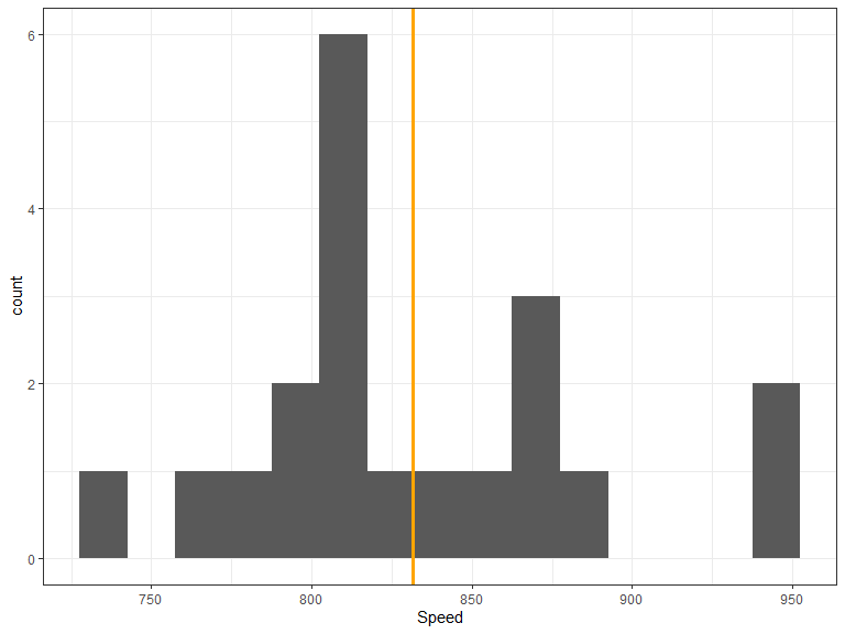
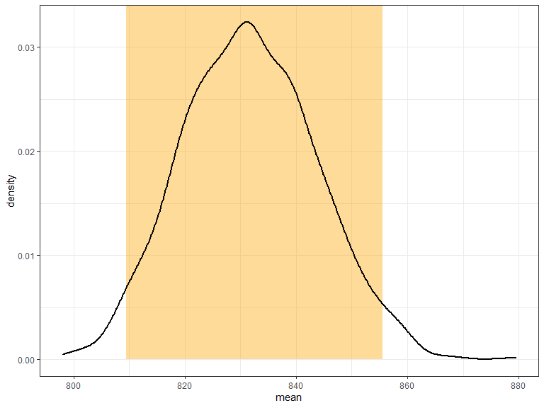
Bootstrapping a confidence interval
- Sample from the data (again and again and again)
- Compute the mean for each sample
- Use the 2.5th and 97.5th percentile of all means as bounds of the confidence interval
Bootstrapping a confidence interval
- Sample from the data (again and again and again)
- Compute the mean for each sample
- Use the 2.5th and 97.5th percentile of all means as bounds of the confidence interval
Bootstrapping a confidence interval
- Sample from the data (again and again and again)
- Compute the mean for each sample
- Use the 2.5th and 97.5th percentile of all means as bounds of the confidence interval
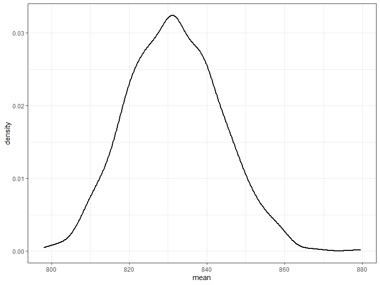
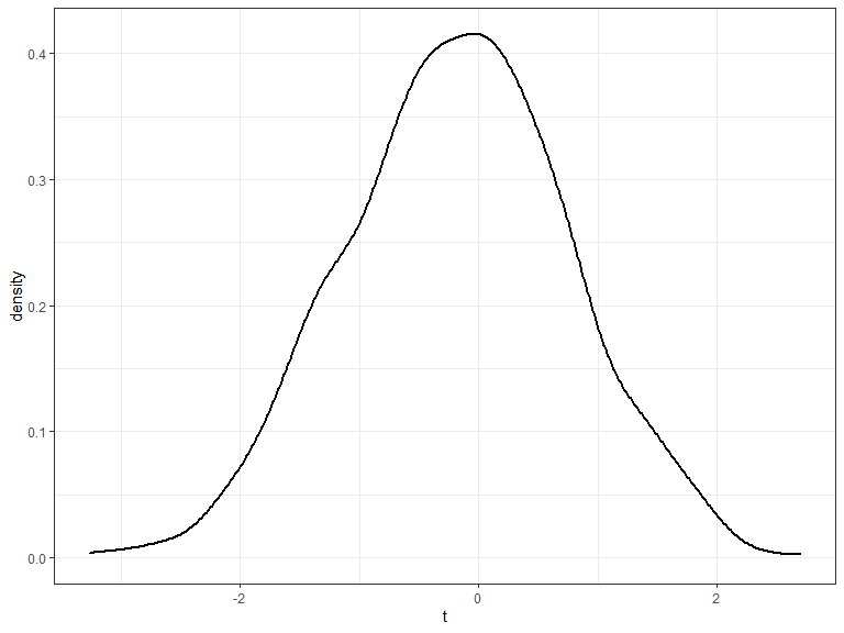
A bootstrap estimate of the p-value
- Bootstrap distribution of means is centred on observed mean.
- This is based on the observed data, i.e. not the null distribution
- Use this to approximate the null distribution.
- Calculate p-value based on number of bootstrap samples at least as far from the null as the observed mean.
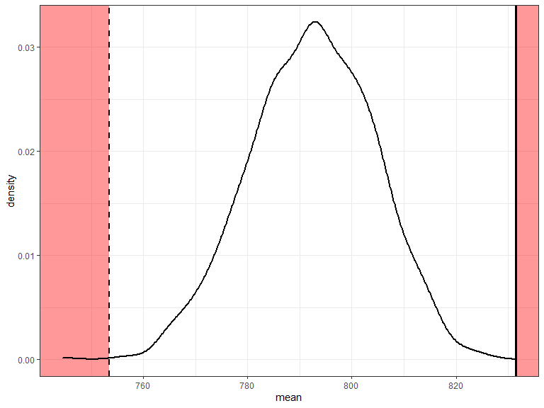
p = 0.001
Studentized Bootstrap
- Instead of using the sample mean \(\bar{x}\) use the t statistic \(\frac{\bar{x} - 792.5}{\hat{\textrm{se}}}\)
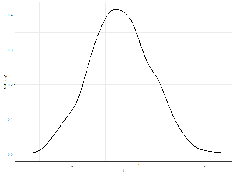
Studentized Bootstrap
Instead of using the sample mean \(\bar{x}\) use the t statistic \(\frac{\bar{x} - 792.5}{\hat{\textrm{se}}}\)
Then proceed as before
Studentized Bootstrap
Instead of using the sample mean \(\bar{x}\) use the t statistic \(\frac{\bar{x} - 792.5}{\hat{\textrm{se}}}\)
Then proceed as before
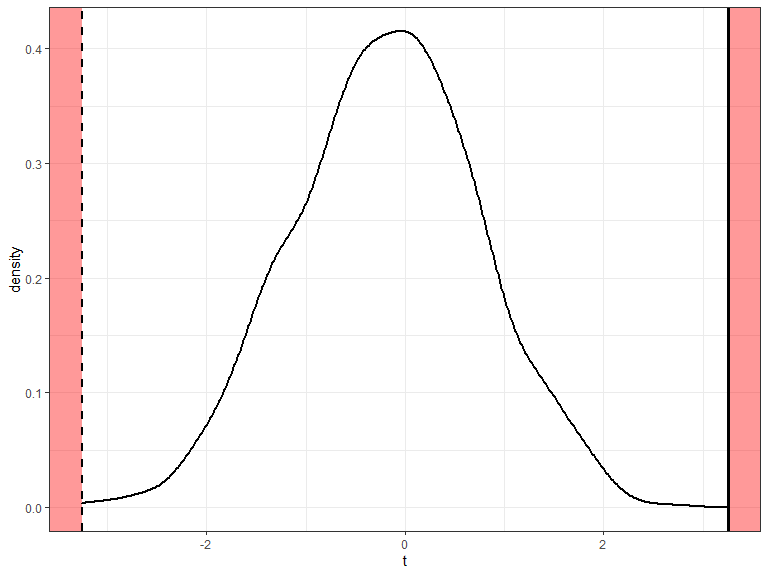
p = 0.001
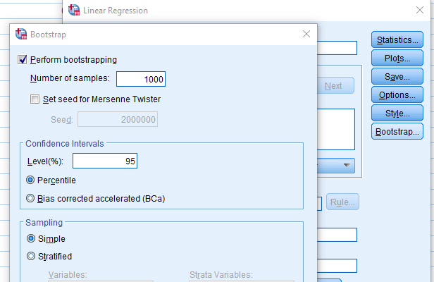
How do I do this myself?

SPSS
- Options for bootstrapping are built into many analysis functions
Thank you